Notes on SuperPoint

SuperPoint: Self-Supervised Interest Point Detection and Description

这是我看的第一篇特征点检测的文章…

这篇文章是 Magic Leap 的。

Motivation

文章的主要贡献给出了一种不需要 human annotation，以 Self-Supervised 训练的 fully-convolutional CNN 来同时学 interest point detectors and descriptors。

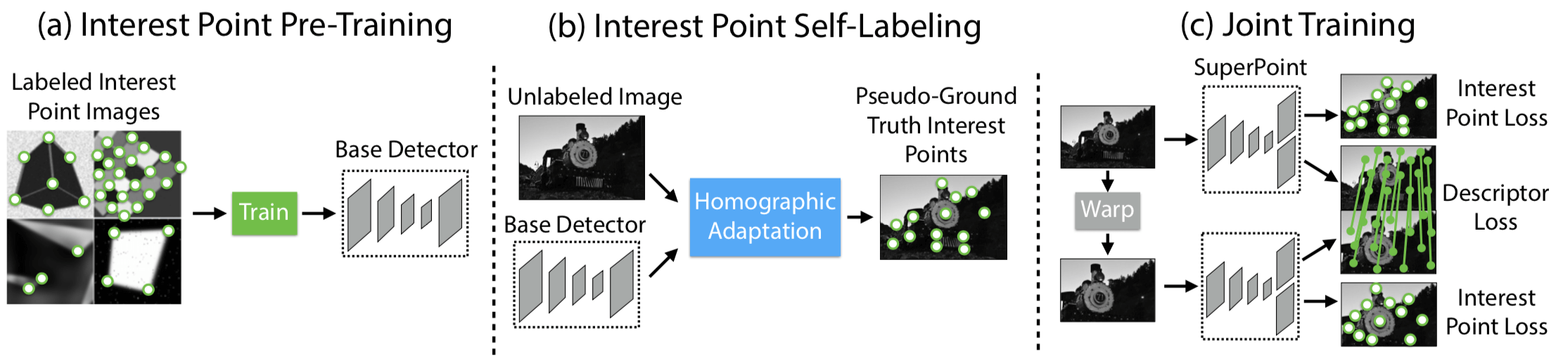
Self-Supervised 是以 From Simple to Complex 的方式实现的，之所以这么做，在于作者相信能够 transfer knowledge from a synthetic dataset onto real-world images，具体步骤如下图所示：

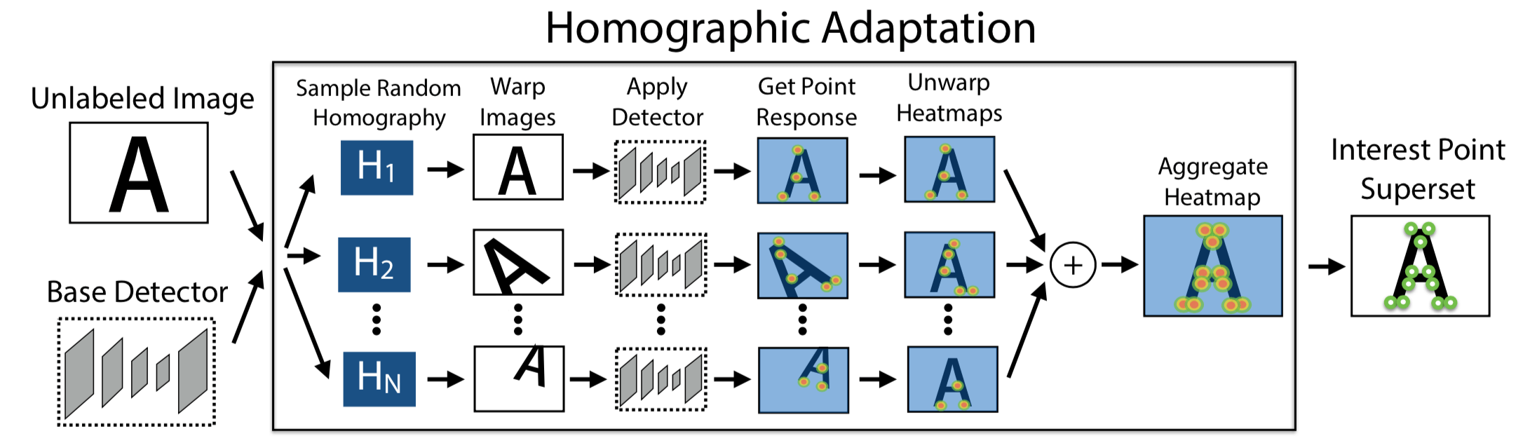
首先是 pre-train an initial interest point detector on synthetic data（这是 From Simple to Complex 的 Simple 阶段），这个阶段得到的 Detector 叫作 MagicPoint；MagicPoint 在 synthetic data 上表现比传统的特征点检测子要来得好，但对于 real images，相比于经典检测子还是会 misses many potential interest point locations. 后面这个能力会通过 Homographic Adaptation 这个 multi-scale, multi-transform technique 来补全（意思就是说作者认为，synthetic data 相比于 real images，缺少 multi-scale, multi-transform，所以 MagicPoint 缺的是在 multi-scale, multi-transform 下的鲁棒性？）
第二步是 Interest Point Self-Labeling，现在 unlabeled image（这是 real images，不是 synthetic data，这是 From Simple to Complex 的 Complex 阶段）上检测出特征点，然后再运用 Homographic Adaptation，就可以得到单应性变换后的特征点。Homographic Adaptation 的核心在于 刻画 repeatability，最后 detectors and descriptors 的 loss 其实惩罚的就是在 repeatability 上表现不好的，而非检测的特征点与 Human Annotated 特征点之间的 Loss。也就是说，之所以能够 Self-Supervised，在于 Loss 由刻画 Prediction 与 Groundtruth 之间的差距，变成了刻画 Prediction 在 Homographic Adaptation 下的 repeatability，也就是 Homographic Adaptation 前后的差距。
最后就是 Joint Training，根据 Loss Function 用 ADAM 优化即可，在优化 Detector 的同时 Description 也学了，Description 就是 CNN 最后的特征表示。

Model

网络结构就是 VGG 的，但因为 SuperPoint 是同时做 interest point detection 和 interest point description，这两个 task 是同时的，共同 share 一部分 computation（传统方式是先做 point Detection，完后了再做 point description），SuperPoint 之所以可以说是同时做，是因为它 Detection 和 description 两个 sub-network 的输出都是 W * H，也就是输入大小，所以 SuperPoint 是做了一个 Dense Output。

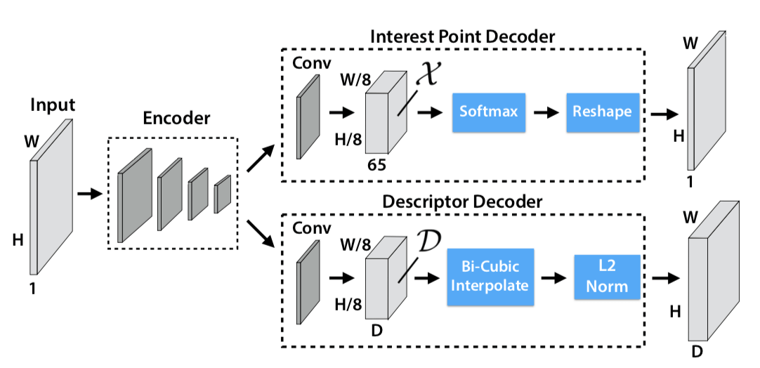
upsampling 没有学习，直接用的插值

对于 Interest Point Decoder，Softmax 之前的特征的尺寸是 $H { c } \times W { c } \times 65$，65 是因为 8 8 下采样一个 Cell 里面对应原来 64 个 Pixel，再加上一个额外的 “no interest point” dustbin，一共 65 个。原图是 W H，现在变成了 W/8 H/8 64，所以变成 W * H 的大小只要 reshape 就可以了

在 Training 阶段，Homographies 是被用来作为提高模型 repeatability 的约束条件 / Loss 来用；在 Test 阶段，Homographies 被拿来当做集成学习多个弱分类器组合成强分类器那样的味道来做，只不过这个组合方式是简单的对在做了单应性变换后检测出来的特征点再反变换回原图的结果的相加，具体公式如下

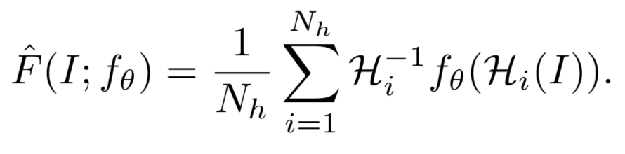
图像表示如下

Loss

注意，Loss 是建立在 $H { c } \times W { c }$ 的 Feature map （8 * 8 下采样）上，而不是在最后跟原图一样大小的 Output 的。

总的 Loss Function 如下：

$$
\begin{array} { l } { \mathcal { L } \left( \mathcal { X } , \mathcal { X } ^ { \prime } , \mathcal { D } , \mathcal { D } ^ { \prime } ; Y , Y ^ { \prime } , S \right) = } \ { \mathcal { L } { p } ( \mathcal { X } , Y ) + \mathcal { L } { p } \left( \mathcal { X } ^ { \prime } , Y ^ { \prime } \right) + \lambda \mathcal { L } _ { d } \left( \mathcal { D } , \mathcal { D } ^ { \prime } , S \right) } \end{array}
$$

interest point detector loss

interest point detector loss 具体如下

$$
\mathcal { L } { p } ( \mathcal { X } , Y ) = \frac { 1 } { H { c } W { c } } \sum { h = 1 \atop w = 1 } ^ { H { c } , W { c } } l { p } \left( \mathbf { x } { h w } ; y _ { h w } \right)
$$

其中

$$
l { p } \left( \mathbf{ x } { h w } ; y \right) = - \log \left( \frac { \exp \left( \mathbf { x } { h w y } \right) } { \sum { k = 1 } ^ { 65 } \exp \left( \mathbf { x } _ { h w k } \right) } \right)
$$

$y { h w }$ 是 label，是特征点在这个 $8 \times 8$ 的 Cell 里面的哪个 pixel 的 label；$\mathbf { X } { h w }$ 是一个长度为 65 的特征向量，里面的每一个数值代表着相应的 pixel 上是特征点的响应值（只是响应值不是概率，经过上式的 softmax 后才是概率值）；上式是典型的 Cross Entropy Loss，因此 interest point detector loss 其实是一个 Cross Entropy Loss。

Y 就是 MagicPoint 在原图上检测出的兴趣点，作为 pseudo groundtruth interest point，X 则是 SuperPoint 网络的 Detector 在原图上检测出的兴趣点，在第一次迭代的时候，X 和 Y 应该是一样的，因为 MagicPoint 就是没有 descriptor head 的 SuperPoint，但随着 SuperPoint 的迭代优化，X 是会发生变化的。这个时候这个 Loss 会去惩罚跟 Y 不一样的 X，也许 X 检出了更多的点呢，这一点合理吗？

虽然 MagicPoint 会 misses many potential interest point locations，但已经算是 performs surprising well on real images 了。所以 MagicPoint 检出的点作为 pseudo groundtruth，后面由 MagicPoint -> SuperPoint，不再努力检测出更多的点，而是致力于 boost repeatability（检测出尽量多的点与检测出的点在 large viewpoint changes 还具有很好的 repeatability 这是两个性质。）

MagicPoint performs reasonably well on real world images 但还不够好，相比于其他经典检测子，但是 Homographic Adaptation 也就是 self-supervised approach for training on real-world images 提高了性能（提高性能不一定非要从减小 Prediction 和 Groundtruth Annotation 的任务中来，也可以是构建其他 Loss，这就是 Self-Supervised 的精髓吧）

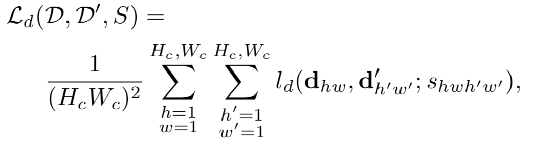
descriptor loss

对于 Description 的 Loss，监督信息是通过 Homographic Adaptation 来实现的，从而完成了的监督学习, 具体计算如下，

其中 $S$ 是一个指示矩阵，指示第 $hw$ 个 cell 是否与 $h’w’$ 个 cell 是 corresponding 的。怎么判断两者是否 corresponding 依据下面这个公式，原图上的特征点做单应性变换后与原图做单应性变换检测出的特征点（先检测后变换，还是先变换后检测的区别），如果一个落在另一个的邻域内，就算是 corresponding 的。

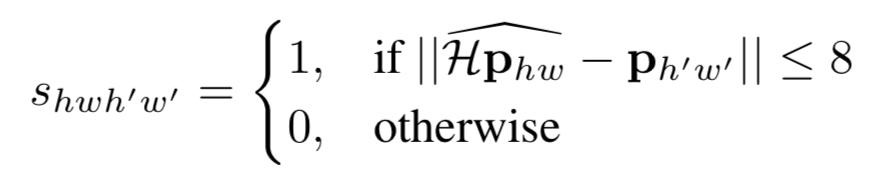
原图上的特征点做单应性变换后与原图做单应性变换检测出的特征点如果在完美的检测和单应性变换下应该是一致的，形式化表示如下。上面的公式其实就是把下面等式两边的两项差距小于 8 的都认为满足这个约束，是同一个点。其实下面这个式子是 repeatability 具体的形式化表示。 repeatability 被刻画成了单应性约束。

$$
\mathcal{ H } \mathbf { x } = f _ { \theta } ( \mathcal { H } ( I ) )
$$

有了 corresponding 关系后，两者之间的 Loss 就可以如下算出来

$$
\begin{aligned} l { d } \left( \mathbf { d } , \mathbf { d } ^ { \prime } ; s \right) & = \lambda { d } s \max \left( 0 , m { p } - \mathbf { d } ^ { T } \mathbf { d } ^ { \prime } \right) \ & + ( 1 - s ) * \max \left( 0 , \mathbf { d } ^ { T } \mathbf { d } ^ { \prime } - m { n } \right) \end{aligned}
$$

这项 Loss 容易理解。如果 s = 1，则表示这两个点是 corresponding 的，那么就是第一个惩罚项非零，惩罚两者的 Description 不够接近；如果 s = 0，则表示这两点是不 corresponding 的，那么就惩罚第二项，惩罚两者的 Description 接近了。其中，$m_p = 1, m_n = 0.2$

Motivation

Model

Loss

interest point detector loss

descriptor loss

Further Reading Material